REVIEW8 | Query Processing
查询处理,看下数据库怎么处理SQL指令字符串的
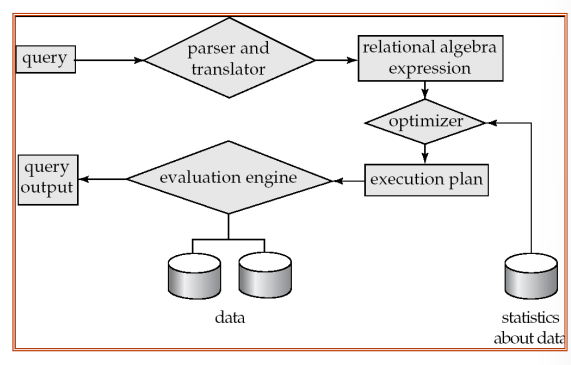
Basic Steps in Query Processing
- Parsing and translation
- 语法检查,并转化为关系代数表达式
- Optimization
- 查询优化,是最重要的一步
- 关系代数通过等价变化进行化简
- 对代数里的每个算子选择合适的算法来实现
- 得到 execution plan,是数据库内部的一种计划语言
- execution plan 告诉引擎每个算子选择什么算法,操作是怎么连接的
- 查询优化,是最重要的一步
- Evaluation
- execution plan交给引擎,开始搜索
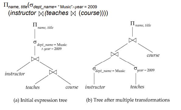
给个 Parsing and translation & Optimization 的例子
select name, title
from instructor natural join (teaches natural join course)
where dept_name=‘Music’ and year = 2009;
execution plan 是从叶子往上执行,右边是初步优化,用到的规则是把选择运算推到了叶子节点,提前选择以减少后续运算量
Measures of Query Cost
磁盘访问时间是cost的大头,是我们讨论的重点,其包括:
- Number of seeks * average-seek-cost
- Number of blocks read * average-block-read-cost
- Number of blocks written * average-block-write-cost
写操作完成后会再读一次来检查,所以写操作的cost远大于读
为方便起见,我们只用磁盘块的读取数量以及寻找次数来衡量,而且省略CPU的cost,以及省略数据写回磁盘的cost,因为流水线模式下临时结果不会被写回磁盘,只有最终的结果才会被写回去,而且我们进行最坏情况估计,假设内存的空间很小
- \(t_T\) - time to transfer one block
- \(t_S\) - time for one seek
Algorithm
Selection
A1 (linear search)
属于 File scan,即扫描所有block,检查所有record
设 \(b_r\) 是关系 \(r\) 占用的block,则
- worst \(cost\) = \(b_r * t_T + t_S\)
- average \(cost\) = \((b_r /2) t_T + t_S\)
如果我们检查的是 key attribute,那么找到了一个就不用往下搜了
A2 (B+-tree index equality on key)
属于 Index scan ,即利用到了索引
该算法是是对主键进行等值查找的情况,找到一个即可
\(Cost\) = \((h_i + 1) * (t_T + t_S)\)
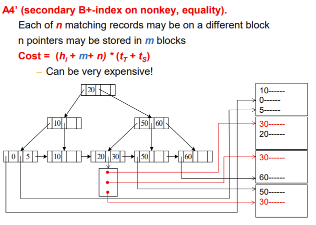
A3 (B+-tree index equality on non-key)
对非主键进行等值查找的情况,可能会有很多个,需要遍历完
\(Cost\) = \(h_i * (t_T + t_S) + t_S + t_T * b\)
上面还是record排好序的情况,如果是乱序的更麻烦
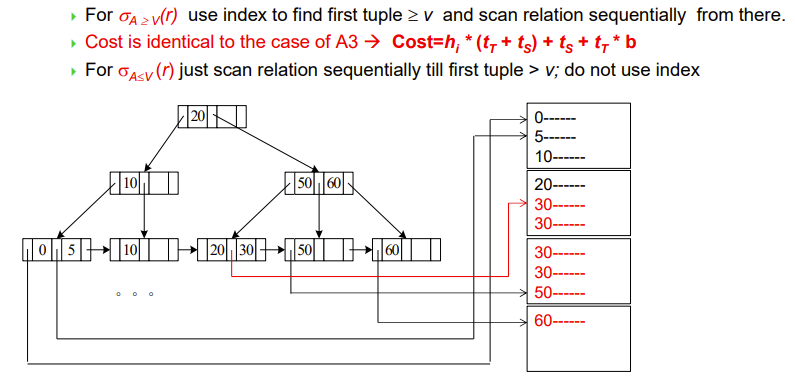
A5 (B+-index index, comparison)
之前都是等值查询,这算法是比较查询,需要分 大于/小于 两种情况
注意我们都是默认file排好序了
- 找出大于V的,就 index 出第一个大于V的,剩下的顺序找到结尾可,不用index
- Cost = \(h_i * (t_T + t_S) + t_S + t_T * b\)
- 找出小于V的,都不用index了,直接从头找,找到大于V的停止即可
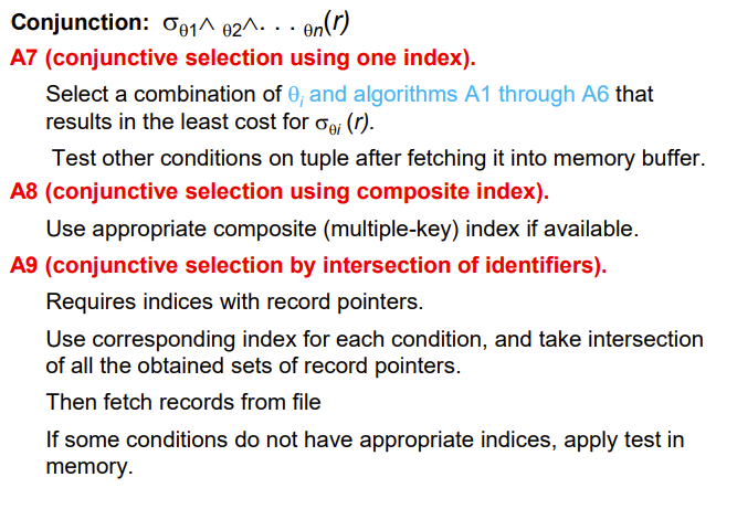
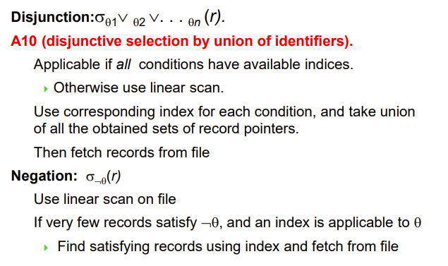
Implementation of Complex Selections
没看,懒得看了
External Sort-Merge
没看,后面再看
上面的算法都是默认file已经排好序了,我们看下怎么去排序
我们考虑的是内存不够大的情况,即需要用到外部排序
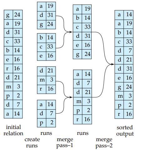
- Create sorted runs(归并段)
- Let \(i\) be \(0\) initially.
- Repeatedly do the following till the end of the relation: 1. Read \(M\) blocks of relation into memory 2. Sort the in-memory blocks 3. Write sorted data to run \(R_i\) ; increment \(i\).
- Let \(N\) be the final value of \(i\) - 这个N是指有几个run
- Merge the runs (N-way merge).
- IF \(N < M\), single merge pass is required (如果归并段少于可用内存页 ) 1. Use \(N\) blocks of memory to buffer input runs, and 1 block to buffer output. Read the first block of each run into its buffer page 2. repeat 1. Select the first record (in sort order) among all buffer pages 2. Write the record to the output buffer. 1. If the output buffer is full, write it to disk 3. Delete the record from its input buffer page. 1. If the buffer page becomes empty then read the next block (if any) of the run into the buffer 3. until all input buffer pages are empty
- If \(N \ge M\), several merge passes are required. 1. In each pass, contiguous groups of \(M - 1\) runs are merged. 2. A pass reduces the number of runs by a factor of \(M - 1\), and creates runs longer by the same factor. 1. E.g. If M=11, and there are 90 runs, one pass reduces the number of runs to 9, each 10 times the size of the initial runs 3. Repeated passes are performed till all runs have been merged into one
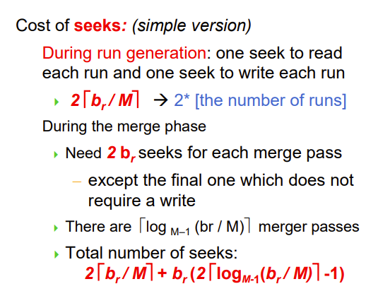
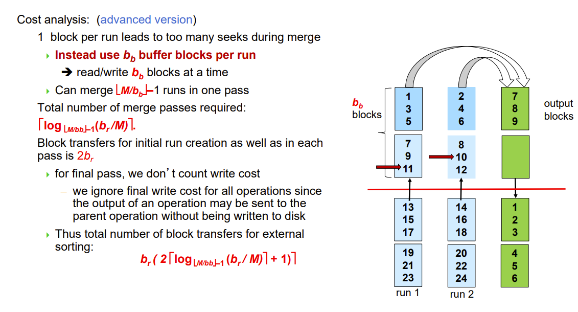
cost分析
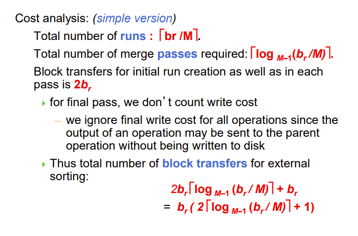
br是数据占的block,M是内存buffer有的block
M-1是一次能归并的block,还有一个留来输出
Join Operation
没看,后面再看
有五种典型算法
- Nested-loop join
- Block nested-loop
- join Indexed
- nested-loop join
- Merge-join Hash-join
Nested-Loop Join
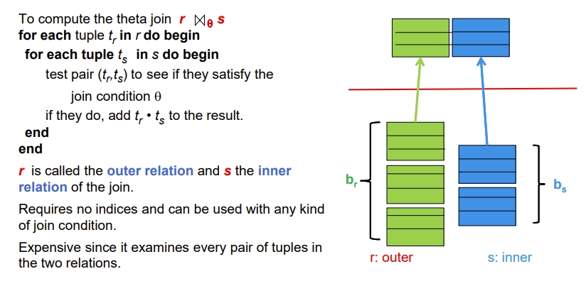
两重循环,遍历r和s的tuple
外循环的叫outer relation,内循环的叫inner relation
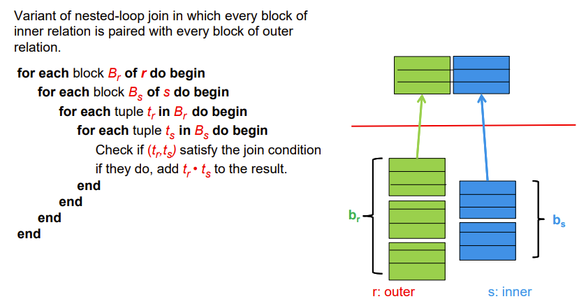
Block nested-loop
循环基本单位改成块,然后块与块再一个嵌套循环
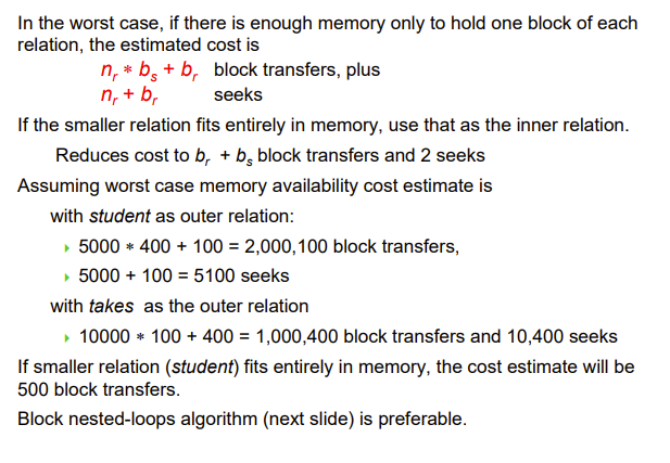
Worst case estimate: $ b_r+b_r * b_s$ block transfers + \(2 * b_r\) seeks
- Each block in the inner relation \(s\) is read once for each block in the outer relation
可见小关系放外循环比较好
Best case: \(b_r + b_s\) block transfers + \(2\) seeks
即内存足够大,r和s一次性进去即可
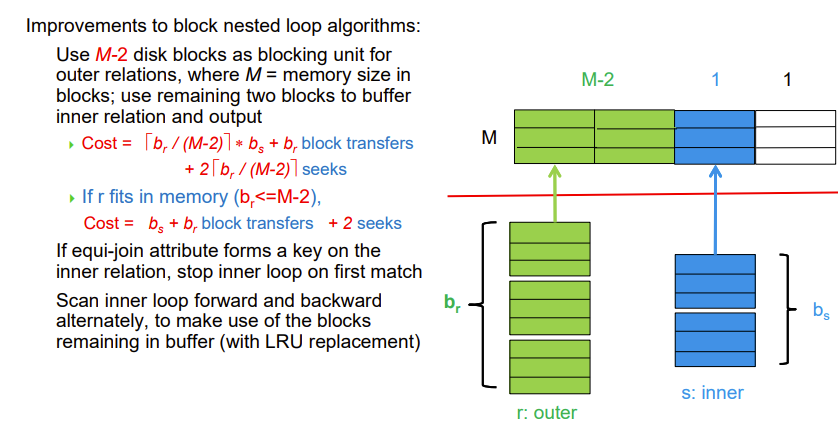
注意,上面是只有2个buffer block的情况,实际上我们有很多buffer block,下面讲多个buffer的情况
Indexed Nested-Loop Join
我们之前的思路都是外循环与内循环一一匹配
我们尝试通过索引替代内循环
- Index lookups can replace file scans if
- join is an equi-join or natural join
- and an index is available on the inner relation’s join attribute
对于每个r的tuple,我们通过索引查找满足条件的s的tuple
Worst case: buffer has space for only one page of r, and, for each tuple in r, we perform an index lookup on s.
Cost of the join: \(b_r (t_T + t_S) + n_r * c\)
- Where c is the cost of traversing index and fetching all matching s tuples for one tuple or r
- c can be estimated as cost of a single selection on s using the join condition.
If indices are available on join attributes of both r and s, use the relation with fewer tuples as the outer relation.

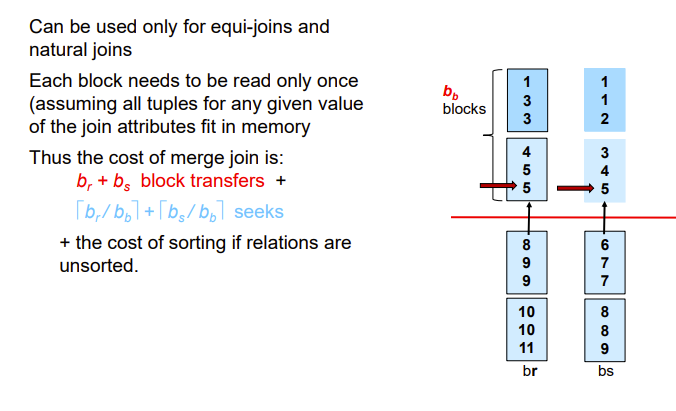
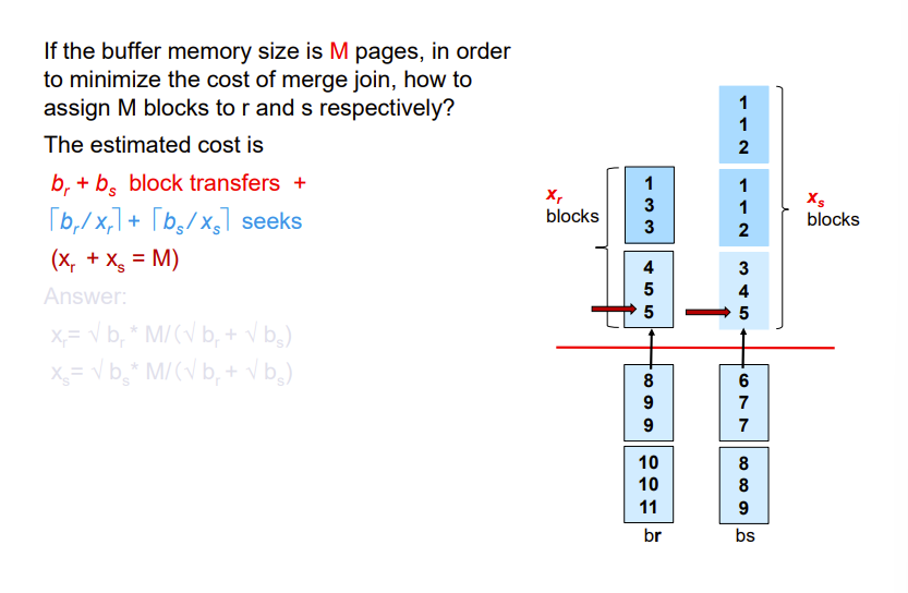
Merge-Join
Join step is similar to the merge stage of the sort-merge algorithm.
Main difference is handling of duplicate values in join attribute — every pair with same value on join attribute must be matched
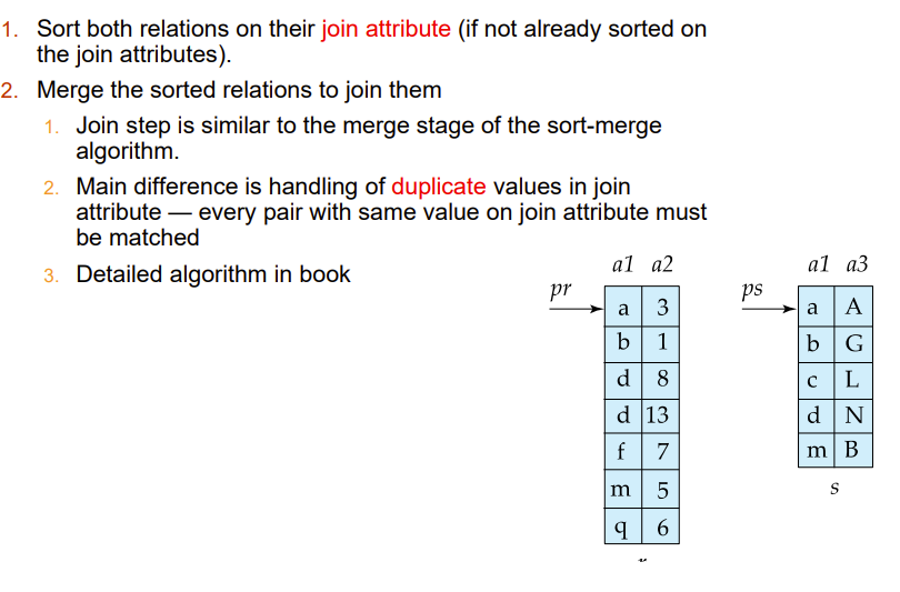
注意这个merge-join需要表先排好序
下面这个方法允许一个表无序

Hash-Join
引入哈希函数,函数值相同的归为一个集合
然后在这个集合内进行两重循环
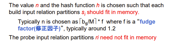
至于哈希函数的稀疏成都取决于buffer多大,至少能让一个集合整体读入
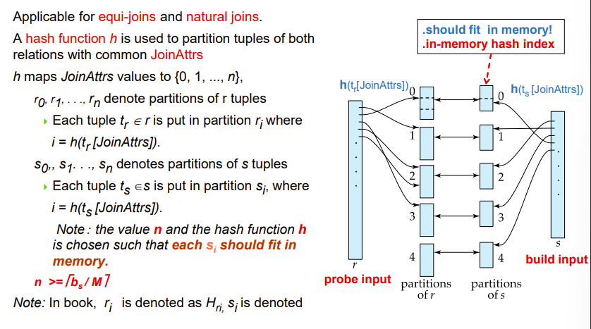
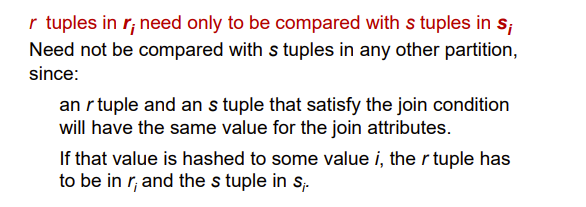
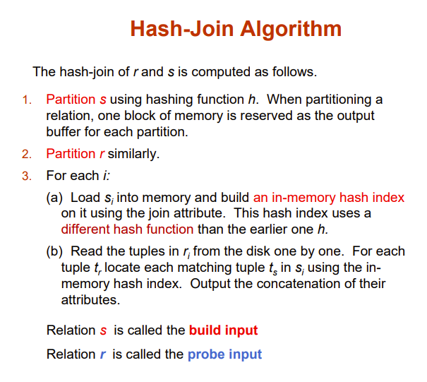
build input是能一次性读入内存的
Recursive partitioning
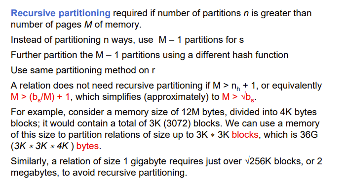
上面那个不等式很重要,决定要不要递归partition
嵌套partition,即patition太大了放不进buffer,就建一个新的哈希函数将patition拆分,还是大就再分别拆分